Measurement of the velocity ratio
of solids and gas in vertical pneumatic conveyor lines

1 Introduction

To calculate the pressure loss, respectively to dimension the different sections of a pneumatic conveying line, the local ratio of the velocities of solid and conveying gas, C = u_S⁄ u_F ≤ 1, is always required [1,2]. This ratio changes in the course of the conveying path. Measurements [3] of the C values of a fine-grained and a coarse-grained bulk material in vertical pipe sections up to the range of very high loads μ =  Ṁ_S ⁄ Ṁ_F are reported below. Given a steady state flow at the measuring point, the settling velocities w_T,ε of particle clouds can then be back-calculated from the determined data and compared with the individual particle settling velocities w_T,0.

The following specifications apply: True velocities are designated by „u_X“, so-called empty pipe velocities by „v_X“. For the gas phase in pneumatic conveying lines, the following then applies, for example, v_F = ε_F ∙ u_F, with ε_F = relative gap volume of the gas. Since ε_F in such systems has values ε_F >~ 0,90, it is generally reasonably accurate to set u_F = v_F. The evaluation of tests in actual practice is normally always based on this assumption.

2 Testing technique

2.1 Test system configuration and test procedure

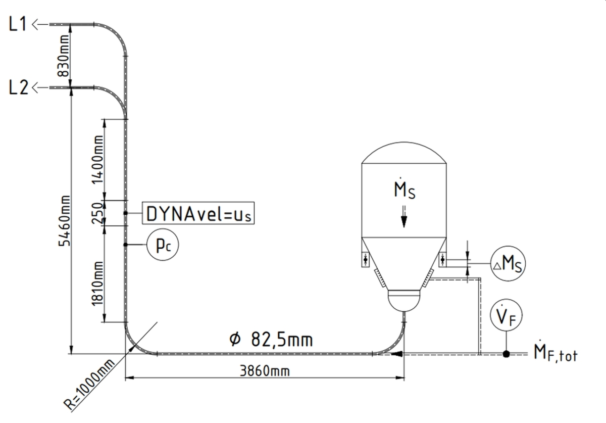
The measurements were conducted on two conveying lines with the inner diameter D_R = 82.5 mm and lengths L_R = 159 m and L_R = 50 m. After injection of the solids, both lines run through the same conveyor pipe to the end of the vertical section in which the measured value acquisition device is installed to determine the C value. The pipes then separate. In the tests presented here, the bulk solids were injected through a downward-discharging pressure vessel with V_B = 2,0 m³ net volume and a large-area gas supply to the cone that assists discharging of the solids. The main part of the conveying gas is fed directly to the beginning of the conveying line. Figure 1 shows schematically the course of the common conveying section of both pipes up to their division and the position of the measuring arrangement contained in it for determination of C.

The pressure vessel feeds the bulk material flow to a horizontal conveying pipe, which is deflected after approx. 3.86 m by a 90° bend with the radius R_U = 1.0 m into a vertical line with the total height H_R ≥ 5.5 m. The arrangement of the installed measuring devices is shown clearly in Figure 1. Their inlet pipe section has an undisturbed length/diameter ratio of (L_zu⁄ D_R) ≅ 22, while that of the outlet pipe section is (L_aus⁄ D_R) ≅ 17. The conveyor section itself consists of a drawn mild steel pipe.

For determining the true solids velocity u_S, the DYNAvel measuring system from DYNA Instruments [4] including the necessary peripherals was used. DYNAvel determines u_S without calibration by means of a transit time measurement. For this purpose, the local capacities that build up due to the bulk material friction in the conveying process are recorded at two measuring points with a defined distance ∆x between them, are compared using a cross-correlation calculation and the resulting transit time difference ∆t is used to calculate the solids velocity u_S = ∆x⁄∆t.

The local gas velocity u_F,C at the measuring point was determined by measuring the gas mass flow
.M_F,tot supplied to the conveying system minus the so-called top/displacement gas flow  .M_F,O by means of the absolute conveying pressure p_C measured directly upstream of the DYNAvel device using the ideal gas law. Details are provided in section 2.3.

The solids throughput .M_S is determined by means of load cells on the basis of both the increase in weight over time of the receiving container at the end of the conveyor section and the decrease in weight of the injecting pressure vessel.

With a constant conveying line pressure difference ∆p_R in each case, the initial conveying gas velocity v_F,A was gradually reduced from high v_F,A-values into the range of the conveying ability limit. The pressure differences ∆p_R were varied in pressure stages of ∆p_R ≅ (1,0 - 2,0) bar. Back pressure of all conveyors: p_G ≅ 1.0 bar. Conveying gas: ambient air with a relative humidity of φ = (50 - 60)%. Operating temperature = solids/gas mixing temperature: T_B ≅ 20 °C.

The particle size distributions of the conveyed bulk materials were checked for changes at regular intervals. If there were any deviations from the original distribution that affected the conveying behaviour, the bulk material was replaced with fresh product. The measured values relevant for the evaluation were always recorded under stable, fully developed operating/flow conditions. All measuring devices are integrated into a data acquisition and evaluation system.

2.2 Analysed bulk solids

The two analysed bulk solids are limestone chippings (LSC) and a limestone powder (LSP) ground from the LSC in a ball ring roller mill. Table 1 compares some characteristic values of these two solids. The limestone powder LSP has an extremely broad particle size distribution, while that of the limestone chippings LSC is relatively narrow.

As the relatively high gas velocities, v_F,A > 10 m⁄s, required to convey the coarse limestone resulted in considerable grain destruction, the LSC had to be replaced after every two bulk material cycles. This considerably limited the number of test runs possible with this material (limited amount of bulk material available).

2.3 Test evaluation

From the definition of the solid/gas velocity ratio, the velocities at the C measuring point are calculated as follows

(1)

The local gas empty pipe velocity v_F,C is calculated as:

(2)

with:  .M_F,tot - total gas mass flow fed to the conveyor system,  .M_F,O - top gas mass flow, which replaces the bulk material volume displaced from the feed vessel and keeps the feed vessel pressure constant,

ϱ_F,C - gas density at the C measuring point.

The following applies for the displacement gas flow:

(3)

with: ϱ_F,B - gas density in the feed pressure vessel.

The gas densities ϱ_F,C and ϱ_F,B are calculated using the ideal gas law from the local absolute pressures p_C and p_B. The relative gap volume ε_F,C at the C measuring point that is required to solve equation (1) can be determined from the continuity equations of the two phases :  .M_S = (1 - ε_F,C) ∙ A_R ∙ ϱ_S ∙ u_S,C and  .M_F = ε_F,C ∙ A_R ∙ ϱ_F,C ∙ u_F,C = A_R ∙ ϱ_F,C ∙ v_F,C. In dimensionless form, this results in:

(4)

When inserted into equation (1) and solved according to C the result is:

(5)

r_V,C =  .M_S/  .M_F ∙ ϱ_F,C ⁄ ϱ_S =  .V_S ⁄   .V_F,C is the volume flow ratio of the two phases at the C measuring point and is better suited to describe the gas/solid interactions, especially at high loads, than μ, compare section 3. It must be noted that in all of the above-described measurements the evaluations were based on mean values over the cross-section of the conveying pipe and mean values over a limited observation period, usually ∆t_mess ≅ (1...2)min.

3 Measurement results

Due to the fact that in practice only the empty pipe gas velocities v_F and the load μ are used, Figure 2 first depicts the approximation C* = u_S,C ⁄ v_F,C instead of C = u_S,C ⁄ u_F,C over the load μ. For both bulk materials, C* can be described in each case by a linear dependence of μ. In the case of the limestone powder LSP, this exceeds the physically non-achievable value of C = 1 at μ ≅ 100. Comparison with Figure 3, which describes the C values calculated with equation (5) dependent on μ, shows that C asymptotically approaches the value C = 1 in infinity. The potency functions depicted in Figure 3 only describe the course of C in the analysed measurement range. The correspondence of C* and C is sufficiently accurate for practical tasks in the range of smaller loads μ, in the case of the limestone powder for example in the range μ <~ 40.

Since the load μ contains absolutely no information regarding the spatial density of the gas/solids mixture ϱ_b,C at the measuring point, i.e. regarding the relative distances of the bulk material particles, it appears to make sense to plot the measurement results in the form C(r_V,C), as r_V,C takes into account the pressure dependence of the measured values, see Figure 4. This likewise does not lead to a reduction in the bandwidth of the measurement results determined. The same applies to the plotting of C against other characteristic values determined from dimensional analyses of the problem.

Evidently, the measured C fluctuations are caused by a different formation/stability of the flow patterns between the 90° elbow at the base of the vertical section and the C-measuring point. In the 90° deflection, the conveying gas and solids become segregated. A pronounced bulk solids strand forms on the outer wall of the pipe, which appear to be more stable in the case of high loads μ or volume flow ratios r_V,C in the further course of the flow than it is in the range of lower values of these characteristic values. At lower loads/volume flow ratios, this strand disintegrates into balls/dunes etc. during the re-acceleration of the bulk material that had been decelerated in the 90° bend, which leads to the measured fluctuating C values. Some calculations for this are presented in the following.

The limestone powder LSP is considered here: its strand thickness at the outlet from the 90° base point elbow is to be evaluated. The two-phase flow is assumed to be incompressible in the conveyor line area under consideration (inlet of base manifold to C measuring point). The solids volume content in a pipe element is calculated from the relative gap volume of the conveying gas to ε_S = (1 - ε_F). In the deflection at the base of the vertical section, the solids are slowed down to half their entry speed (realistic value for fine-grained bulk solids): u_S,U,out = u_S,U,in ⁄ 2 = u_S,C ⁄ 2. Its re-acceleration takes place on the way to the C measuring point. For the volume content of the solid at the manifold outlet, the value ε_S,U.out = 2 ∙ ε_S,C is derived from its continuity equation  .M_S ⁄ (A_R ∙ ϱ_S) = ε_S,U,out ∙ u_S,U,out = 
ε_S,U,out ∙ u_S,C ⁄ 2 = ε_S,C ∙ u_S,C. Since both the sought ε_S,U,out and the ε_S,C back-calculated from the measurement results are mean values over the conveying pipe cross-section, the ε_S,U,out must be further divided into a dense strand portion ε_S,Str and a low-solids portion ε_S,0 outside the strand in order to determine the strand thickness. From the continuity equation  .M_S ⁄ (ϱ_S ∙ u_S,U,out) = ε_S,U,out ∙ A_R = ε_S,Str ∙ A_Str + ε_S,0   A₀ and ε_S,Str ≅ k ∙ ε_S,SS with ε_S.SS = ϱ_SS ⁄ ϱ_S, ϱ_SS = loosely piled bulk density, k = correction factor for the strand density, the following is the result, taking into account ε_S,U,out = 2 ∙ ε_S,C for the share of the strand cross-section in the total conveying pipe cross-section:

(6)

Table 2 compares the relevant calculations for two LSP tests with very different loads μ. For ε_S,0 = 0 and k = 1 the strand cross-sections listed in Table 2 are obtained. These decrease for ε_S,0 > 0 and increase for k < 1. Along the vertical conveying section between the foot point bend and the C measuring point, it is evident that considerable changes in the flow characteristics with corresponding effects on the C measurement are possible.

Additionally, Figure 5 shows the course of the dependence of the relative gap volume ε_F,C of the conveying gas at the C measuring point plotted against the current load μ.

The back-calculated ε_F,C measured values of the LSC fit in well with the measured values of the LSP shown in the diagram and, as required, run at μ 0 into the value ε_F,C 1. A simple potency equation therefore does not adequately describe the behaviour of ε_F(μ) in the range of low loads μ.

4 Settling velocity of particle swarms

For the settling velocity w_T,ε of a particle accumulation/particle swarm relative to the conveying gas, the following derives from equation (1) with

(7)

By definition, the determination of w_T,ε requires a temporally and spatially constant flow condition in the measuring section. In the tests presented here, this is only guaranteed with the fine-grained limestone powder LSP. For this reason, only results with this bulk material are presented below. Results of comparable measurements are represented in the literature, e.g. in the form of

⇥(8)

(9)

Other approaches are possible and are known in the literature. Figure 6 shows the back-calculated settling velocities w_T,ε of the LSP as a function of the load μ. These show significant differences in the curves of the measurement series carried out with respectively different constant pressure loss/length unit ∆p ⁄ L_R i.e. with different pressure p_C at the C measuring point.

The reason for this is that the forces from particle flow, weight and buoyancy that have to be taken into account for their effect on the particles in the case of the single particle settling velocity w_T,0 must be supplemented by the particle/particle and particle/pipe wall forces/interactions in the case of the particle swarm. These are usually modeled summarily as frictional resistance (λ_S,ε∝∆p_R ⁄ L_R ).

It follows from the above calculation approaches for the swarm settling velocity w_T,ε that w_T,ε in accordance with the function

(10)

is dependent on the size of the delivery pipe diameter. A larger pipe diameter leads to a lower settling velocity w_T,ε under comparable operating conditions (μ,...), as this results, among other things, in a reduced number of wall and particle impacts. All LSP measurements carried out here are therefore only valid for the analysed pipe diameter D_R = 82.5 mm.

In Figure 7, the LSP measurement results are plotted non-dimensionally in the form  

Reynold-No Re_T,ε = w_T,ε ∙ d_S,50 ∙ ϱ_F ⁄ η_F = f (FroudeNo Fr_R,C = u²_F,C ⁄(g ∙ D_R)). This results in a linear dependency Re_T,ε(Fr_R,C). The Re_T,ε number is thereby formed with the median value d_S,50 of the LSP particle size distribution, while the Fr_R,C number is formed with the gas velocity u_F,C at the C measuring point.

The relatively wide range of measuring points encompasses their different loads μ and also the influences of the different flow forms along the measuring section. The advantages of the representation depicted in Figure 7 are, firstly, that the Fr_R,C number already contains the w_T,ε-dependence on the conveying pipe diameter, D_R, equation (10), i.e. Figure 7 can also be applied to other pipe diameters (investigations in this regard on a DN 50 vertical section are currently underway), and secondly, that even when using the easily determined empty pipe gas velocity v_F,c instead of the true velocity u_F,c it is possible to make a simple/rough estimate of the swarm settling velocity w_T,ε.

Comparisons with other bulk solids are possible, inter alia, via the dimensionless characteristic values Ar or (w_T,ε ⁄ w_T,0), e.g. equations (8) and (9).

It must once again be emphasised that the measuring method described here can only be used to determine averaged C or w_T,ε values over the cross-section of the conveying pipe, which although reflecting the influences of the respective flow patterns, but do not describe these conditions quantitatively. In order to determine the effects/characteristic values of different flow forms, e.g. of balls, strands etc. of solids, flow-specific calculation models are required, the characteristic values of which must be determined in tests with the specific flow forms occurring in the conveying pipe, compare e.g. [7, 8].