Basic considerations for pneumatic conveying against high back pressures

1 Introduction

Various plant manufacturers are currently planning process plants for special bulk materials with operating pressures of p_G = (40 – 50) bar, which are to be fed with finely ground solids by pneumatic conveying systems. For energetic and economic reasons, higher loads are required of these conveyor systems, μ = M·  _S / M·  _F >20, with: M·  _S, M·  _F = mass flows of solids (S) and conveying gas (F). It is well known that larger loads result in a reduced energy requirement for the solids transport. Compared to the loads of pneumatic conveying systems working with almost atmospheric pressure, i.e. systems conveying against p_G ≅ 1 bar, this does not appear to present a problem. However, the fact that the gas phase of the 2-phase flow of gas/solids is compressible is often underestimated or not sufficiently taken into account. Increasing conveying pressure or back pressure results in an increasingly stronger compression of the conveying gas and thus, at a given solids throughput M·  _S, in a decrease in the local distances between the bulk solids particles, i.e. in a mixture compression, and thus in an increase in the local solids volume fraction. Ultimately, this also results in a larger required conveying gas mass flow M·  _F to provide the required conveying gas velocity for a given solids mass flow M·  _S and thus in a reduction in the maximum load μ that can be achieved.

Since the load μ along a conveying section L_R is constant, it does not provide any information about the profile of the local spatial density of the gas/solids mixture ϱ_b in the pipe and therefore also provides no specific information about the locally occurring flow patterns. As a general rule, for describing the gas /solid interactions, i.e. particle /particle and particle /pipe wall collisions with corresponding effects on the delivery pipe pressure loss Δp_R, other parameters, e.g. the use of the volume concentrations of one of the two phases, are more suitable. In the case of the high-pressure conveying systems considered below, a number of simplifications can be made, as will be shown in the following.

With high back pressures, the conditions at the start of the delivery line are critical, as this is where the highest pressure p_in and therefore the lowest gas velocity v_F,in occur. If at this point the mixture density exceeds a limit value ϱ_b,crit, that corresponds approximately to that of the loose bulk density ϱ_ss, the solids then form a plug that fills the entire cross-section of the conveyor pipe, totally blocking it due to wedging.

The following paragraphs first describe in detail the dependence of the conveying gas velocity v_F on the pressure ratios p_in/p_out prevailing in the pipe, followed by that of the load μ(p_in) and the limit load μ_crit specified by ϱ_b,crit and discuss their consequences. Next, some suitable and proven economic design variants for pneumatic solids injection at high back pressures are presented.

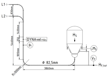
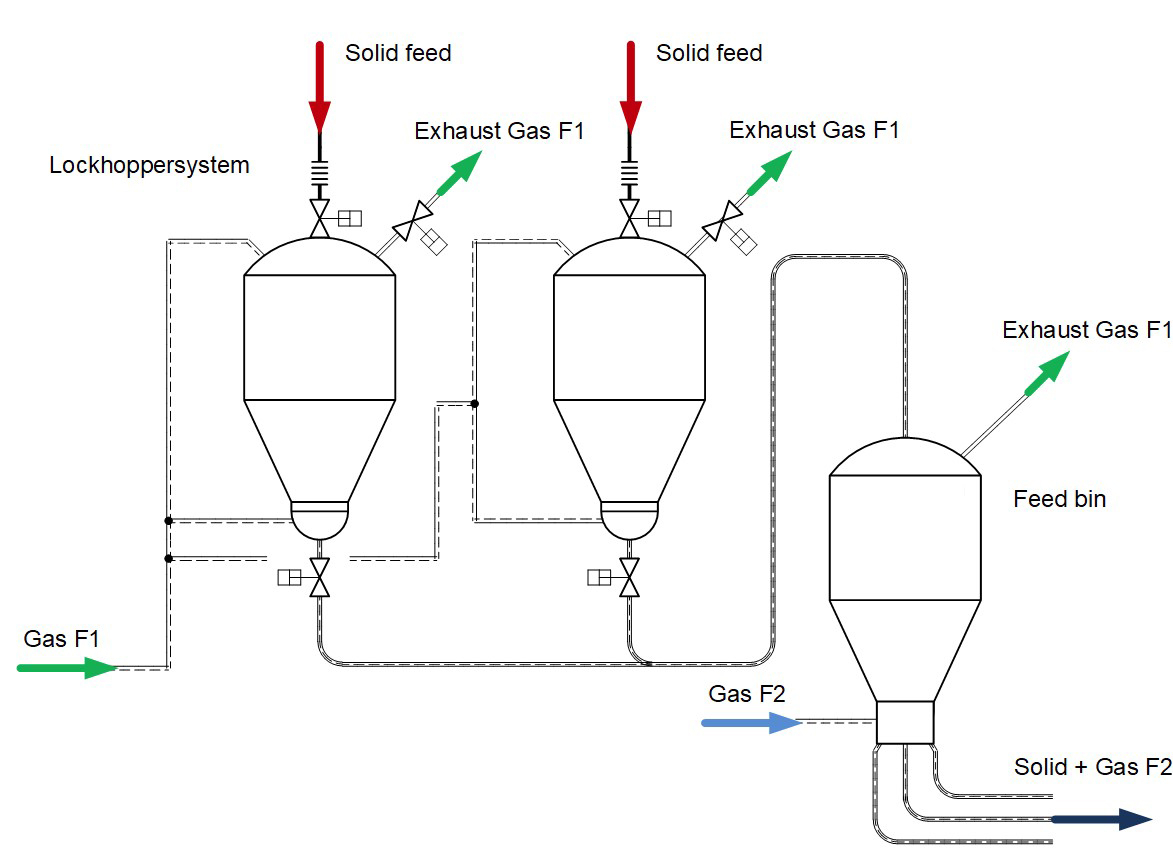
Further considerations are based on the example of the pneumatic conveyor system shown in Figure 1, which transports from the “lock hopper system” to the “feed bin” = feed into the process plant.

The following stipulations apply: True velocities are indicated by “u_x” and so-called empty pipe velocities by “v_x”. For the gas phase in pneumatic conveying systems, the following applies, for example: v_F = ε_F·u_F, with ε_F = relative gap volume of the gas. As ε_F has values ε_F ≳ 0.90 in such systems, it is generally possible to specify u_F = v_F with reasonable accuracy. The relative gap volume ε_F corresponds to the gas volume fraction in the pipe element ΔV_R that is currently under consideration, while the corresponding volume fraction of the solid material is represented by ε_S. The following therefore applies: ε_F + ε_S = 1.

2 Conveying gas velocities

The conveying gas velocities at the beginning (in) and end (out) of an (unstaggered) conveying section with a constant mixture temperature T_M along the pipe follow with the ideal gas law from

⇥(1)

⇥(2)

Example 1:

v_F,in = 10.0 m/s, Δp_R = 1.0 bar, p_G = 1.0 bar

⇥

Example 2:

v_F,in = 10.0 m/s, Δp_R = 1.0 bar

(alternatively: 5.0 bar), p_G = 40.0 bar  

alternatively:

At the high conveying pressures/counterpressures considered here, an approximately constant conveying gas velocity v_F is established along the conveying section. This means that at the selected gas inlet velocity v_F,in the flow pattern of the gas/solids mixture is largely maintained over the entire conveying distance. Critical conveying conditions, e.g. plug formation in the case of fine-grained bulk solids, therefore no longer resolve themselves. In atmospheric pressure operation, the considerable gas expansion would support the plug dispersion process.

3 Pressure dependence μ(p) of the load

For a given solids mass flow rate M· _S the continuity equation of the conveying gas for the load is as follows:

⇥(3)

In the following, the operating conditions at the critical starting point of the conveying pipe (in) are considered and the condition of the gas is described using the ideal gas law

⇥(4)

with: ϱ_F  - gas density,

p_in - absolute pressure at the beginning of         the conveying line,

R_F   - specific gas constant,

T_M  - absolute mixture temperature,

Furthermore, the initial conveying gas velocity v_F,in is divided into a minimum velocity v_F,in,min and the distance to this minimum velocity Δv_F,in that is currently selected for the system design. The following applies:

⇥(5)

v_F,in,min is the minimum conveying gas velocity below which no solids can be conveyed. It can be derived from conveying diagrams showing the respective bulk material to be conveyed. As an example, Figure 2 shows the pressure dependence of the solids throughput M· _S relating to ground biomass for systematically varied conveying gas velocities v_F,in at two different conveying pressure differences Δp_R at the conveying section D_R = 54,5 mm x L_R = 155,3 m, back pressure p_G = 1.0 bar. The ordinate intersections of the M· _S curves correspond to the minimum velocities v_F,in,minat the respective pressure difference Δp_R, i.e. each pressure loss curve Δp_R is assigned a v_F,in,min value. If measurements are carried out with the same operating settings on a conveyor section with a larger pipe diameter D_R , this generally leads to larger v_F,in,min values. This special behaviour is specific to each individual solid. The dependence of the minimum velocity v_F,in,min for any given bulk material must be determined experimentally and can be represented with sufficient accuracy for practical use using the empirical power approach

⇥(6)

In Equation (6), the gas density ϱ_F,in has a decisive influence. The greater this is, the greater the ability of the conveying gas to carry solids. Using the ideal gas law, the following applies

⇥(7)

with: K_v,k,ℓ - solid-specific constants/exponents,

            to be determined by experiment.

Equation (7) describes the relevant influencing variables of pipe diameter D_R, type of gas R_F, operating temperature T_M, conveying pressure p_in, type of bulk material and the condition of the gas, i.e. also the influence of local altitude, relative gas humidity φ etc. Details regarding the minimum velocity can be found in [1, 2].

Note: For a selected pressure difference Δp_R, the conveying diagram in Figure 2 provides a simple way of determining the energetically optimum operating point = state of minimum specific energy demand P_spez = (P_V / (M· _S · L_R))_min - usually stated in [kWh/(t ·100m)]. This corresponds to the point of contact of the tangent from the coordinate origin with the respective curve Δp_R = konst. At this operating point, the associated maximum possible load μ_max occurs. It is evident that the corresponding conveying gas velocities v_F,in, especially in the case of fine-grained bulk solids and high conveying pressures, are too close to the conveying limit v_F,in,min to be of use for practical operation designs.

For a specific calculation task (→ solid and conveying gas given), the following results from equation (7)

⇥(8)

p_in is to be used as the absolute pressure. By applying a double logarithmic plot of v_F,in,min(p_in) at D_R = konst. or v_F,in,min(D_R) at p_in = konst. the exponents k and ℓ, as well as the constant K_v* can be determined from their respective gradients. The exponents determined in this way are in the range (k,ℓ) ≅ 0…1. It can be seen that the (k,ℓ) values are systematically dependent on the flow behaviour of the bulk solids currently being conveyed [1, 2]. Equation (8) is currently confirmed by practice up to p_in ≅ 20 bar.

The distance Δv_F,in of the conveying gas velocity from the current applicable minimum velocity v_F,in,min, equation (5), can be freely selected taking into account the characteristic curve/behaviour of the lock system and the requirements of the downstream plant equipment, e.g. with regard to freedom from pulsation. If pneumatic conveying, i.e. transport of solids takes place at gas velocities v_F,in ≥ v_F,in,min + Δv_F,in then

⇥(9)

can be applied, see Figure 3.

From the measurement results in Figure 2 and Figure 3, the resistance coefficients for calculating the conveying pipe pressure loss Δp_R can also be determined. This is discussed in section 7.

The equations (4, 5, 7) inserted into equation (3) provide the pressure dependence of the load

⇥

⇥(10)

It can be seen from this equation this that for given boundary conditions (→ M·  _S, D_R, Δv_F,in) the possible load μ in each case decreases approximately inversely, proportionally with increasing conveying pressure p_in. The counteracting term p_in^ℓ that describes the pressure dependence of the minimum velocity has an exponent ℓ ≅ 0.5 for fine-grained bulk solids and is only of minor influence.

4 Critical load μ_crit

The pressure dependence of the load μ that is described by equation (10) provides no information as to whether it can actually be attained in practice.

At the inlet to a pneumatic conveying section charged with an increasingly large mass flow M·  _S a limit state (crit) is reached at a certain M·  _S. In this state the solid particles fill the entire pipe cross-section and are in permanent contact with each other, i.e. they form a solid structure that cannot be compressed any further. This condition corresponds approximately to that of a loosely piled heap and can be described, for example, by the relative volume proportion of the solid material in the pipe element under consideration

⇥(11)

with: ε_s, ε_F - volume fractions of solids and gas,

(ε_s +ε_F) = 1

      ϱ_b,crit- critical bulk density at the start of
the pipe,

        ϱ_ss- loosely heaped bulk density of the
bulk material,

          ϱ_s- particle density of the solid, it is often identical with the specific density of the solid

In order to achieve the desired conveyance with the solids volume fraction at the beginning of the pipe, the condition

⇥(12)

must therefore be fulfilled. The current solids volume fraction at the conveying pipe inlet follows from the continuity equations of the two phases M·  _S = ε_s,in·A_R ·ϱ_S · u_s,in  and M·  _F = (1 - ε_s,in ) · A_R · ϱ_F,in · u_F,in 

= A_R · ϱ_F,in· v_F,in , leading to

⇥(13)

Consideration of the equations (5, 9) and the explanations in section 3 and in [1] lead with u_s,in =Δv_F,in to equation (14)

⇥(14)

Evaluation of equation (12) by inserting equations (11) and (14) yields the critical = maximum possible load μ_crit of the planned conveyance. The following applies:

⇥(15)

Note: In the above considerations, see equation (11), the gas density ϱ_F,X was neglected compared to the densities ϱ_b,x and ϱ_s. If very light bulk solids and very high conveying pressures occur at the same time, the solids volume fraction ε_s,X should be calculated using the more accurate approach

ϱ_b,x = ε_S,X · ϱ_s + (1 - ε_S,X) ·ϱ_F,X as follows

⇥(16)

In equation (15), the variables ϱ_F,in  and v_F,in,min are dependent on the conveying pressure p_in, i.e. it is not possible to make a direct μ_crit calculation without knowing the pressure loss |Δp_R | of the conveying section (L_R, D_R) at a given back pressure p_G. In practice, the desired operational setting is used to first calculate the conveying distance and the resultant load μ, and its achievability is then checked with the critical load μ_crit determined using equation (15). As starting values for this iteration, the parameters corresponding to the back pressure p_G= p_out can be used. Any necessary corrections then require a change in the operating conditions in the conveying pipe, e.g. by increasing the distance Δv_F,in  to the conveying limit v_F,in,min etc. The iteration is stable.

Figure 4 presents an example of a special fine-grained hard coal dust with the characteristics of mean particle diameter d_S,50 = 27 μm, solid ≅ particle density ϱ_s = 1650 kg/m³, bulk density ϱ_ss = 550 kg/m³ as well as the associated constants of v_F,in,min equation (8) k = 0, ℓ = 0,35, K_v= 4.0 bar ^0.35· m/s showing the dependence of the critical = maximum load μ_crit for the constant distance Δv_F,in = 5.0 m/s to the current conveying limit v_F,in.

The conveying gas is air, the operating temperature T_B = 20 °C. It can be seen that, for example, the maximum possible load of μ_crit ≅ 34 kg_s/ kg_F at p_in = 10 bar falls to μ_crit≅ 7 kg_s/ kg_F at p_in = 50 bar, The exponent of the power function balancing the calculated values in Figure 4 has a value n = 0.918 that is close to 1, as was to be expected on the basis of the previous explanations, equation (10).

Figure 5 shows, for the same application, the dependence of the load μ_crit on the distance Δv_F,in at conveying pressures p_in = 10 bar and 50 bar.  μ_crit increases, as can already be seen from equation (15), with greater Δv_F,in. As this raises the distance to the conveying limit, the gas/solids mixture can be compressed more strongly.

As a general rule, the greater the back pressure p_G = p_out and thus the conveying pressure p_in, the lower the maximum possible limit load μ_crit. Increasing the distance Δv_F,in of the conveying gas velocity relative to the conveying limit Δv_F,min,in leads to higher critical loads μ_crit. The limit curves μ_crit(p_in) are specific to the particular solid.

Alternative approach: As can be seen from equation (12), the volume fraction of the solid ε_S,in at the beginning of the conveying pipe must remain lower than/equal to a critical volume fraction ε_s,crit in order to achieve pneumatic conveyance. If ε_s,X  is replaced on both sides of equation (12) by ϱ_b,x / ϱ_s (→corresponding to equation (11)) and ϱ_s is removed, the following results:

⇥(17)

i.e. the bulk density ϱ_b,in of the solids entering the conveyor pipe must not exceed a limit value ϱ_b,crit ≅ ϱ_ss  (→ loosely tipped bulk density of the current bulk material). Based on the above assumptions, the following applies for density ϱ_b,in  from the continuity equation of the solid:

⇥(18)

If A_R is back-calculated from the continuity equation of the conveying gas M·  _F = A_R · ϱ_F,in· v_F,in and introduced together with equation (18) into equation (17), this results, after a few elementary conversions, in the dependency equation (15) for the permitted or maximum possible load μ_crit (→ this also results with permissible simplifications when using equation (16)). The presented approaches are therefore largely identical

5 Energetic consideration

The back pressure of the infeed, p_G, to the “feed bin” is determined by the downstream process system. This means that the pressure generator used to compress the gas flow M·  _F to the pressure p_in = p_G +  | Δp_R | needs the power Pv.

Generally, | Δp_R| << p_G under the operating conditions considered here, which means that P_V is hardly determined by the pressure loss Δp_R of the actual conveying section, but is essentially governed only by the size of the gas mass flow M·  _F. For an (idealised) isothermal compression (→ permanent cooling of the compression chamber), the following then applies, e.g.:

⇥(19)

with: p₀, T_F,0 = 1.0 bar, 20 °C, intake suction

              condition.

Practical calculations show that there are optimum conveying pipe diameters D_R in which the energy requirement P_V due to the pipe diameter D_R (→ a reduction in diameter leads to an increase in | Δp_R| and thus also in p_in) and also due to the gas mass flow M·  _F (→ a reduction in diameter leads to a reduction in M·  _F and the other way round) is minimized. Calculations show that the total energy requirement P_V is increased to a lesser extent by increasing the pressure loss | Δp_R| than by increasing the gas mass flow rate M·  _F. The aim of a system design must therefore be to reduce the gas mass flow M·  _F to a level required for the stable attainment of the downstream process (→ distance Δv_F,in). General tendency: smaller conveying pipe diameters are preferable. This optimisation is specific to both the solids involved and the type of compressor. It is always necessary to check the permissible limit load μ_crit.

Example: A hard coal conveyor system with M·  _S = 18.0 t/h, L_R = 50 m, p_G = 40 bar, D_R,1 = 50 mm leads to a pressure loss Δp_R,1 = 3.00 bar. A reduction in the pipe diameter with the same Δv_F,in to D_R,2 = 40 mm results in a pressure loss Δp_R,2 = 5.34 bar. With equation (19) the following applies:

  ⇥(20)⇥

For the operating data given above, the following extremely optimistic value is calculated for the selected Δv_F,in :

Independently of the planned system concept, it follows from the considerations presented here that the systematic optimisation of energy expenditure is obviously a sensible approach to the system design.

6 Gas exchange in the conveying system

If an inert gas F1, compare Figure 1, is used for conveying solids from the “lock hopper system” to the “feed bin” for reasons of safety engineering or explosion protection, but an oxidising gas medium F2 for heat generation, e.g. air, oxygen, carbon dioxide or water vapour, is used  for the feed into the process plant, e.g. a gasification plant, the gas flow F2 mixes at the outlet of the “feed bin“ with the gas flow F1, as this splits into the exhaust gas flow M·   _F1,Abgas and the gap gas flow M·  _F1,ϵ at the head of the “feed bin”. The volume fraction ϵ_F,feed of the gas F1 that arises as the gap volume of the bulk material in the “feed bin” is conveyed with the solid to its outlet (→ u_s = u_Fapplies) and mixes there with the gas F2. The gas mass flow M·  _F1,ϵ can be calculated using the continuity equations of the two phases involved as follows

⇥(21)

with: ϱ_F1  - density of gas F1 at pressure p_G.

Note: In moving bulk quantities of solids, the relative gas gap volume ϵ_F is generally greater than it is in a stationary bulk quantity (→ ϵ_F,feed) and the process of feeding into a container can lead to further loosening or fluidisation of the bulk solids, especially in the case of fine-grained materials.

These effects and pressure differences over the height of the “feed bin” must be taken into account separately.

It is not possible to prevent the mixing of gases F1 and F2 at the outlet from the “feed bin” in the design variant shown in Figure 1. It can only be eliminated, if necessary, by suitable flushing with F2 gas upstream of or integrated into the “feed bin”. The F1/F2 mixture from the flushing process must then be discharged separately.

Example: Under consideration is a gasification plant with a solids throughput of M·  _S = M·  _S,feed = 18.0 t/h of pulverised hard coal with the parameters particle diameter d_S,50 = 27 μm, solids density ϱ_s= 1650 kg/m³, bulk density ϱ_ss= 550 kg/ m³, pressure in the “feed bin” p_G = p_feed= 40.0 bar, and operating temperature T_S = 20 °C.  The F1 gas used is CO₂ with ϱ_CO2, 1.842 kg/m³ at 20 °C, 1 bar. Using equation (11), the resulting value for the relative void volume of the gas in the “feed bin” is ϵ_F,feed = 1 - ϱ_ss/ ϱ_s = 1 – 550 kg m³/ 1650 kg/m³ = 0.666. The density of the F1 gas at the operating pressure p_G is: ϱ_F,1 = ϱ_CO2(20°C,1.0 bar) . p_G /p_O =1842 kg/m³ · 40.0 bar / 1.0 bar = 73.68 kg/m³.   Equation (21) then provides the F1 gas mass flow in the gap volume of the downward-moving bulk solid as:

This gas flow must be included in the design of the process reactor. In practice, as indicated above, the involved M·  _F1,ϵ value will be somewhat greater than calculated here [3].

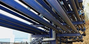
7 Required extent of test work

In order to be able to carry out the examinations described in sections 2, 3 and 4, it is necessary to know or determine by means of experimentation not only the dependency v_F,in,minfor the respective bulk solids, but also the dependency for determining the conveying pipe pressure loss Δp_R. For an unknown/new bulk material, this at least requires measurements on two conveyor sections of the same length, running as parallel as possible, i.e. geometrically similar conveying sections L_R,1= L_R,2 with very different diameters D_R,1≠ D_R,2, compare Figure 6. At least two conveyance characteristic curves (Δp_R,1, Δp_R,2) = konst. must be recorded on both pipes all the way down to the conveyance limit v_F,in,min. The pressure differences Δp_R,1 and Δp_R,2 should be the same in both conveying sections, but should be as far apart from each other as possible. Details on the procedure can be found in [2 ,4] and other sources.

The data then available can be used to back-calculate the dependencies of the minimum velocity characterising the respective bulk solids, as well as the resistance coefficients describing the pressure loss of the pipe. The latter can be performed using different models, e.g. the λ_S-standard model or company-specific approaches, compare [1, 4, 5] and other sources.

8 Design variants

The high back pressures in pneumatic conveying systems mentioned here naturally occur not only in gasification plants but also in other processes, e.g. in the charging of blast furnaces with pulverised coal as a heat transfer and reduction medium. The feeding / lock systems use pressure vessels only.

The “lock hopper system” is usually designed as a parallel configuration of two feeders (→ one feeds, while the other is being filled, i.e. quasi-continuous operation), but could also be designed as a series configuration of two feeders arranged one above the other, i.e. absolutely continuous operation. Both processes have their advantages and disadvantages. The latter solution generally results in a very high overall installation height. Depending on the design, the bulk material is often fed from the feed bin into the downstream reactor in parallel at several feed points, see Figure 1. Figure 7 shows an example of a system for injecting coal into a blast furnace. Typical conveying pressures range up to p_in≅ 20 bar. From the distributor below the “buffer vessel” (= “feed bin”) the coal can be distributed in parallel to any number of outgoing conveying pipes.

The solids throughput M· _S is regulated via the top pressure in the “buffer vessel”. Compared to the design of a feed bin with, for example, multi-cone discharge, which is difficult to implement in terms of construction and strength verification, the design of the buffer vessel with integrated distributor shown in Figure 7 appears to be advantageous. This design allows easy adaptation to downstream gasification/reactor systems of various designs, as the number of conveying pipes leading from the manifold can be individually customised from 1 … n. A tried and tested resistance equalisation of the “n“ individual pipes leaving the distributor allows the same or also defined different solids flow rates in these pipes. [7].