A simple sampling method for VRMs

1 Introduction

Because of the low specific energy consumption and simple compact design of vertical roller mills, their usage is becoming widespread in the cement industry for finish grinding of cement raw material, coal and clinker. Today, in order to produce the final product, dynamic air-classifiers are built on the top of vertical roller mills, evolving from the edge (Brundiek, 1989), and to reduce the high power consumption caused by the internal pneumatic material transportation, this system has been entirely or partially replaced by the external mechanical recirculation system (Feige, 1993).

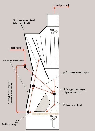
In these systems (Fig. 1), the route of the particles starts with fresh material feeding to the table. Due to the centrifugal force of the rotating table, particles are pushed into the grinding zone between table and rollers and the material crushed under high compression forces leaves the table. After that, the table discharge material is swept up through a dynamic separator by high speed gas flow.

During the pneumatic transport within the mill, the gas behaves like a physical classifier which depends on mill design, operating conditions, and material properties such as size and density starts to be effective on the particles. The fine material is transferred to the separator, while the coarse material recycles back to the system externally. Depending on some obstacles in the mill and sudden expansion of the flow area in which the linear air velocity drastically drops down, the coarse and heavy particles within the stream falls back onto the table which acts as a secondary classifier before the real classifier (Schonbach, 1988).

This article deals with a new sampling method developed to evaluate the separate performances of the classification and grinding sections of the VRM having the compact design. In this study, to solve the mass balance around the VRM, second and third classification sections are assumed as a single stage and they are called the separator. If a representative sample can be collected from the total grinding table feed and product with a crash stop, particle size distributions and tonnages of the streams of separator feed and reject can be estimated using mass balance techniques.

2 Sampling and experimental studies

In order to prove that the sampling method can solve the sampling problem of the VRM, an industrial survey was carried out, and performance evaluation of the circuit was conducted by using the data gathered from the survey.

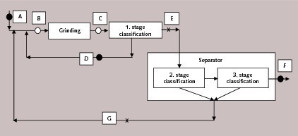
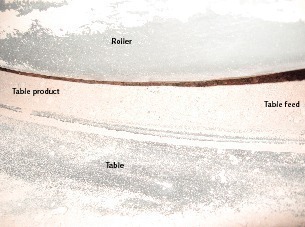
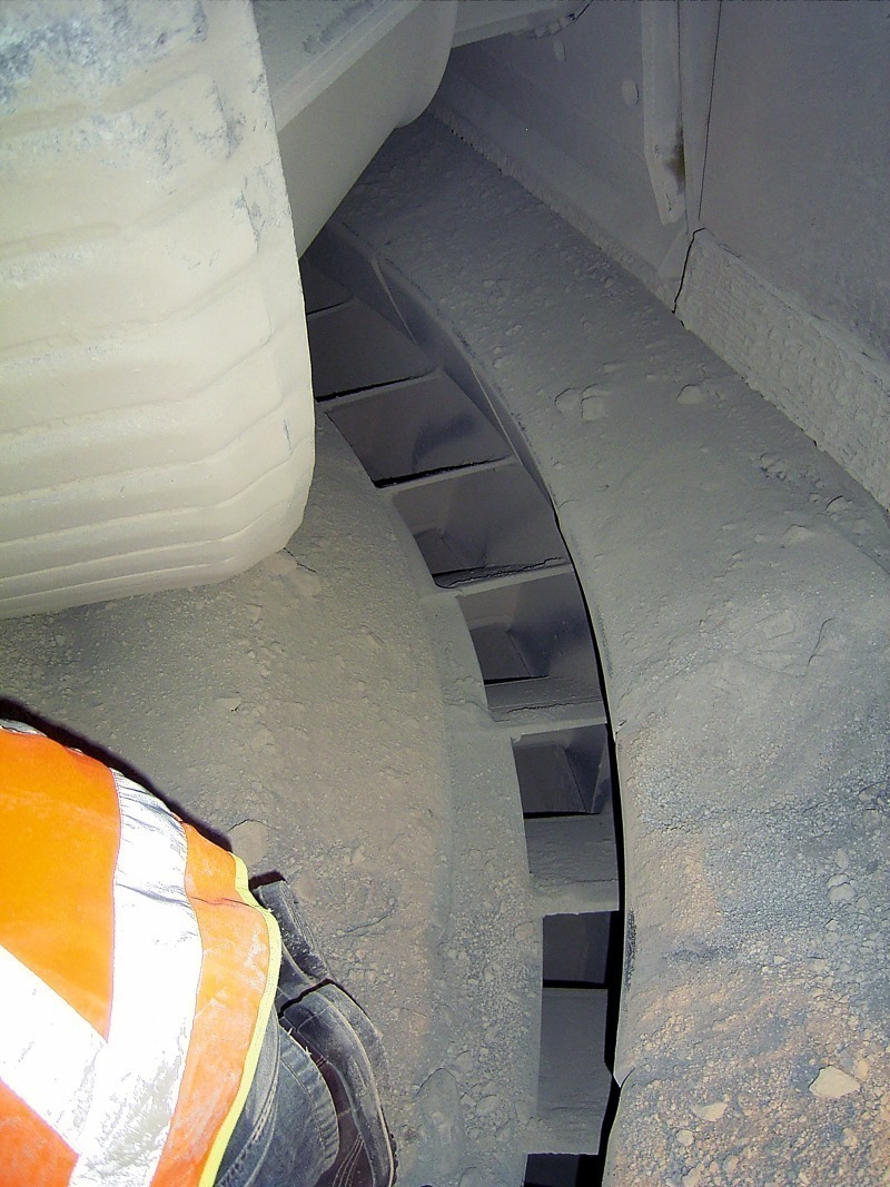
During the survey, streams which are marked with “•” in Figure 2 (A: fresh feed, D: 1^st stage classification reject (external circulating load), and F: final product) are outer streams and can be easily sampled from their own flow points. In addition to those, to solve the mass balance of the system, the total feed and product of the grinding table were sampled after crash stop (points B and C marked with “•”). The materials just before and after the rollers were assumed as the total table feed and product respectively (Fig. 3). In order to calculate the particle size distributions and the tonnages of the separator feed (point E) and reject (point G), the tonnages of streams B and C are required. Since the tonnages of the outside streams were recorded in the control room, the inside streams (point B and C) can be calculated using Equation 1 (Tamashige et al., 1991):

C = 3600 · Z · γ · h · B · ϑ⇥(Eq. 1)

C = Table capacity (t/h)

Z = Number of roller

γ = Bulk density of compressed material (t/m³)

h = Final bed thickness of the material (m)

B = Rollers width (m)

υ = Circumferential speed of table on grinding zone (m/s)

After the sampling studies, size distributions of all samples were determined by dry sieving and laser sizing down to 1.8 µm. Since some of the material remained as flakes in the table product the samples were tumbled in a Ø 70 × 50 cm drum for a complete disagglomeration. The technical and operational parameters of the VRM are given in Table 1.

The industrial survey raw data gathered in order to show that the sampling methodology is successful or not to solve the mass balance problem around the VRM is given in Figure 4.

3 Data reconciliation and mass balance

According to the simplified flow sheet given in Figure 2, for the steady-state operating condition of the system, mass conservation equations can be written as

B - A - D - G = 0⇥Eq 2

Bb_i - Aa_i - Dd_i - Gg_i = 0⇥Eq. 3

C - E - D = 0⇥Eq. 4

Cc_i - Ee_i - Dd_i = 0⇥Eq. 5

E - F - G = 0⇥Eq. 6

Ee_i - Ff_i - Gg_i = 0⇥Eq. 7

B - C = 0⇥Eq. 8

A - F = 0⇥Eq. 9

Upper cases: tonnage of the streams in Fig. 2

Lower cases: mass fraction of the i^th size in the streams in Fig. 2

In this system, after additional sampling points (table feed, B, and table product, C) by using five particle size distribution data, two measured tonnages and one calculated tonnage, unknown tonnages and particle size distributions of “E” and “G” streams (Fig. 2) could be estimated. The solution of the system can be performed from the join node of the total mill feed to the first stage classification node or revers by resolving the mass conservation equations 2 to 9. Using raw data, according to node by node solution, the mass conservation equations give different results.

This situation addresses the necessity of reconciliation of the measurements. For this purpose, the problem can be described as a minimization problem of the sum of squares of differences between measured and reconciled process variables. One of the common and simple solution methods of the constrained optimization problems is the L­agrange multiplier method which consists of creating a new function (ℓ) that has to be optimized by linking the constraint functions (Ω) which has new variables (λ, Lagrange multiplier) with the criterion function (f). When the optimization problem is defined as:

{ m x i n f (X)⇥Eq. 10

  subject to

  Ω (X) = 0

then the general form of Lagrange function is:

ℓ (X) = f (X) + ∑ λ_i Ω_i (X) ℓ (X)

                                  _i

= f (X) + ∑ λ_i Ω_i (X)⇥Eq. 11

                           _i

Because the aim of this study is to solve the sampling problem of VRMs and not to choose the best data reconciliation method, the mass balancing and data reconciliation procedure were simplified by converting the non-linear system with measured and unmeasured variables into a linear system with all measured variables step by step. For this purpose, firstly unknown data sets were eliminated from Eq. 2 to Eq. 9. At that step, one known data set (tonnage and particle size distribution of the stream D) was unavoidably eliminated. After elimination for the first step, the criterion (eq. 12) and constraint functions (eq. 13) can be given as:

f (f_i, a_i, c_i, b_i)

= [f_i - f_im]² + [a_i - a_im]² + [c_i - c_im]² + [b_i - b_im]²⇥Eq. 12

Ω (f_i, a_i, c_i, b_i) = C [c_i - b_i] - A [f_i - a_i] = 0⇥Eq. 13

The integration of Eq. 12 and 13 into Eq. 11 gives:

ℓ (f_i, a_i, c_i, b_i, λ) = [f_i - f_im]² + [a_i - a_im]² + [c_i - c_im]²

+ [b_i - b_im]² - λ (C [c_i - b_i] - A [f_i - a_i])⇥Eq. 14

i: reconciled percentage of the i^th size

im: measured percentage of the i^th size

The minimization of ℓ and f functions is obtained when the partial derivatives of the Lagrange function (eq. 14) with respect to each independent process variables (f_i, a_i, c_i, b_i) and Lagrange multiplier (λ) are equalized to zero.

δ_ℓ/δ_fi = 2_fi - 2f_im + λA = 0  f_i = f_im - λA/2⇥Eq. 15

δ_ℓ/δ_ai = 2_ai - 2a_im + λA = 0  a_i = a_im + λA/2⇥Eq. 16

δ_ℓ/δ_ci = 2_ci - 2c_im - λC = 0  c_i = c_im + λC/2⇥Eq. 17

δ_ℓ/δ_bi = 2_bi - 2b_im + λC = 0  b_i = b_im - λC/2⇥Eq. 18

δ_ℓ/δ_λ = A [f_i - a_i] - C [c_i - b_i] = 0⇥Eq. 19

Integrating the equations from Eq. 15 to 18 into Eq. 19, it can be written as

λ = [A(f_im - a_im) - C(c_im - b_im)]/[A² + C²]⇥Eq. 20

Using the equations from 15 to 18 and 20, the percentages of the size of the sampled streams can be reconciled. After that, the reconciled data and raw data of stream D are used for estimation of the particle size distributions of E and G. Using the first step results, the system is turned into a linear system with all measured variables. In the second step of the conciliation procedure, all obtained reconciled and estimated data in first step are assumed as initial condition. In the final stage, the criterion (Eq. 21) and constraint functions (Eq. 22-24) can be written as,

f (f_i, a_i, c_i, b_i, d_i, e_i, g_i) = [f_i - f_im]² + [a_i - a_im]² +

[c_i - c_im]² + [b_i - b_im]² + [d_i - d_im]² + [e_i - e_im]² + [g_i - g_im]²

+ [d_i - d_im]² + [e_i - e_im]² + [g_i - g_im]²⇥Eq. 21

Ω₁ (b_i, a_i, d_i, g_i) = Bb_i - Aa_i - Dd_i - Gg_i = 0⇥Eq. 22

Ω₂ (c_i, d_i, e_i) = Cc_i - Dd_i - Ee_i = 0⇥Eq. 23

Ω₃ (e_i, f_i, g_i) = Ee_i - Ff_i - Gg_i = 0⇥Eq. 24

When Eq. 21-24 are integrated into the general form of the Lagrange function, the function is given as

ℓ (f_i, a_i, c_i, b_i, d_i, e_i, g_i, λ₁, λ₂, λ₃) = f (f_i, a_i, c_i, b_i, d_i, e_i, g_i)

+ λ₁ Ω₁ + λ₂ Ω₂ + λ₃ Ω₃ + λ₁ Ω₁ + λ₂ Ω₂ + λ₃ Ω₃⇥Eq.25

At that point, the partial derivatives of Eq. 25 are equalized to zero, and same methodology of the first step is applied for the second step. At the end of the calculations, basic equations can be given as:

a_i = a_im + λ₁ A/2⇥Eq. 26

b_i = b_im + λ₁ B/2⇥Eq. 27

c_i = c_im + λ₂ C/2⇥Eq. 28

d_i = d_im + (λ₁ + λ₂) (D)/2⇥Eq. 29

e_i = e_im + (λ₂ + λ₃) E/2⇥Eq. 30

f_i = f_im + λ₃ F/2⇥Eq. 31

g_i = g_im + (λ₁ + λ₃) G/2⇥Eq. 32

After the linear system of three equations with three unknowns given in the below is solved, the results are integrated with the equations from Eq. 26 to 32. This step is the end of the reconciliation procedure.

φλ₁ - (D²/2) λ₂ - (G²/2) λ₃ + γ = 0⇥Eq. 33

(D²/2) λ₁ + θλ₂ - (E²/2) λ₃ - α = 0⇥Eq. 34

(G²/2) λ₁ - (E²/2) λ₂ + ωλ₃ - ß = 0⇥Eq. 35

Because some parameters are too long in equations 33 to 35, they are renamed as follows.

γ = Bb_im - Aa_im - Dd_im - Gg_im

α = Cc_im - Dd_im - Ee_im

β = Ee_im - Ff_im - Gg_im

φ = - (B² + A² + D² + G²)

                       2

θ = (C² + D² + E²)

                  2

ω = (E² +  F² + G² +)

                2

4 Results and discussion

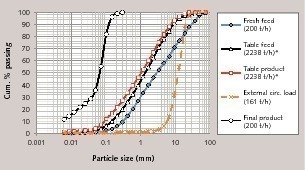
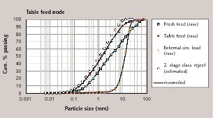
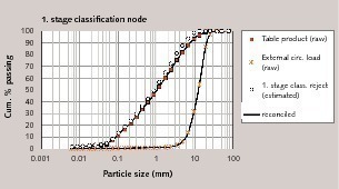
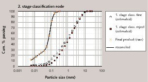
After reconciliation procedure, the raw and mass balanced particle size distributions for each node are given in Figure 5, 6, and 7. The data shows that, a high amount of material was transported pneumatically i.e. the table product size distribution is very close to the first stage classification fine (Fig. 6). Additionally, it is clearly shown from Figure 4 that only about 7 % material of the table product is recirculating externally. For this case, the total recirculating material is 2038 t/h and the circulating load is approximately 1000 %. Schonback (1988) mentioned that the circulating load for roller mills changes between from 500 to 2000 %. Many researchers also indicate that all closed circuit high compression mills (VRM, HPGR, Horomill) have a high circulating load (Aydoğan and Benzer, 2011; Aydoğan and Ergün, 2010; Reyes-Bahena, 2010).

The efficiency curve of a separation unit in closed circuit grinding applications is very important criteria for performance evaluation and modelling. For this reason, this sampling methodology gives critical information about grinding and classification steps of the VRM.

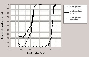
Based on mass balance results, efficiency curves of the separation units were plotted (Fig. 8).The parameters of the efficiency curves, such as cut-size (d₅₀), corrected cut-size (d_50c), by-pass and the imperfection value (I=(d_75c-d_25c)/2d_50c), are given in Table 2.

As a result of the efficiency curves, imperfection value of the second stage separation is seen as a little bit higher when it is compared with high efficient dynamic air classifiers used in ball mill applications (Gunlu, 2006; Altun and Benzer, 2014). For closed circuit HPGR application with high efficient dynamic air classifiers in cement grinding, imperfection values of the corrected efficiency curves were reported between 0.35 and 0.41 (Aydoğan and Ergün, 2011). Considering the dust load of the second stage classification, which is 4.85, it can be said that this value is not too high.

The bypass value of the second stage is also seen as acceptable for a dynamic air classifier, on the other hand it should not be forgotten that in this study second stage classification contains dynamic air classifier and secondary natural air classification. In the sampled VRM, a huge amount of material transported to the second stage but a relatively huge amount of air is also used for transportation. Because of that, when the dust load for this survey is compared with other closed circuit high compression milling (HPGR, Horomill), this value is not so far away from the common value.

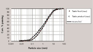
As can be seen from Figure 9 the table product and feed are very close to each other, it also explains the huge amount of circulation load.

5 Conclusions

This study shows that the mass balance of VRMs can be solved by sampling of the total mill feed and product from under the rollers. In this study, data reconciliation and unknown data estimation procedure performed with very simple method to show that if a representable sampling is carried out, the system can be easily mass balanced.

This methodology will give very important data to overcome the obstacles of the modelling and performance evaluation of VRMs. Moreover increasing data sets by this sampling method, the effect of the operating and design parameters on each unit operation and overall performance of VRMs can be demonstrated.